1D Fourier transform
[ ]:
import numpy as np
import matplotlib.pyplot as plt

from deconvoluted import fourier_transform
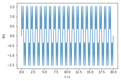
Suppose we want to compute the 1D fourier transform \(F(\nu)\) of a function \(f(t)\). Let us generate a signal which is a superposition of a signal with \(\nu_1 = 1\) Hz and \(\nu_2 = 3\) Hz:
[9]:
t = np.linspace(0, 20, 201)  # 20 seconds
nu_1 = 1
nu_2 = 3
f_t = np.sin(nu_1 * 2 * np.pi * t) + np.sin(nu_2 * 2 * np.pi * t)

plt.plot(t, f_t)
plt.xlabel(r'$t$ / s')
plt.ylabel(r'$f(t)$')
plt.show()
Taking the transform is now simply a matter of calling fourier_transform:
[10]:
F_nu, nu = fourier_transform(f_t, t)
[11]:
plt.plot(nu, F_nu)
plt.xlabel(r'$\nu$ / $s^{-1}$')
plt.ylabel(r'$F(\nu)$')
plt.show()
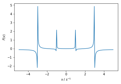
As expected, we find resonances at \(\nu_1 = 1\) Hz and \(\nu_2 = 3\) Hz.
We could also perform the transform using angular frequency instead:
[12]:
F_omega, omega = fourier_transform(f_t, t, convention=(1, -1))
[13]:
plt.plot(omega, F_omega)
plt.xlabel(r'$\omega$ / rad $s^{-1}$')
plt.ylabel(r'$F(\omega)$')
plt.show()
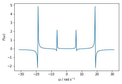
Now our resonances are at \(\omega_1 = 2 \pi\) and \(\omega_2 = 6 \pi\) instead.